Analysis of movies - IMDb dataset

We will look at a subset sample of movies, taken from the Kaggle IMDB 5000 movie dataset
movies <- read_csv(here::here("data", "movies.csv"))
glimpse(movies)
Besides the obvious variables of title, genre, director, year, and duration, the rest of the variables are as follows:
gross: The gross earnings in the US box office, not adjusted for inflationbudget: The movie’s budgetcast_facebook_likes: the number of facebook likes cast memebrs receivedvotes: the number of people who voted for (or rated) the movie in IMDBreviews: the number of reviews for that movierating: IMDB average rating
Use your data import, inspection, and cleaning skills to answer the following:
- Are there any missing values (NAs)? Are all entries distinct or are there duplicate entries?
There are no missing values; after dropping all observations with at least one missing value, the number of observations still remained the same. We observe that 53 movie tites had duplicates - 52 movie titles had one duplicate while the title “Home” had 2 duplicates.
# Cursory glance
movies <- read_csv(here::here("data", "movies.csv"))
glimpse(movies)
## Rows: 2,961
## Columns: 11
## $ title <chr> "Avatar", "Titanic", "Jurassic World", "The Avenge…
## $ genre <chr> "Action", "Drama", "Action", "Action", "Action", "…
## $ director <chr> "James Cameron", "James Cameron", "Colin Trevorrow…
## $ year <dbl> 2009, 1997, 2015, 2012, 2008, 1999, 1977, 2015, 20…
## $ duration <dbl> 178, 194, 124, 173, 152, 136, 125, 141, 164, 93, 1…
## $ gross <dbl> 7.61e+08, 6.59e+08, 6.52e+08, 6.23e+08, 5.33e+08, …
## $ budget <dbl> 2.37e+08, 2.00e+08, 1.50e+08, 2.20e+08, 1.85e+08, …
## $ cast_facebook_likes <dbl> 4834, 45223, 8458, 87697, 57802, 37723, 13485, 920…
## $ votes <dbl> 886204, 793059, 418214, 995415, 1676169, 534658, 9…
## $ reviews <dbl> 3777, 2843, 1934, 2425, 5312, 3917, 1752, 1752, 35…
## $ rating <dbl> 7.9, 7.7, 7.0, 8.1, 9.0, 6.5, 8.7, 7.5, 8.5, 7.2, …# First glance; data types for each variable seem appropriate
# Check for missing values
movies_nomissing <- movies %>%
drop_na()
# We see that after dropping all observations with at least one missing value, the number of observations remain the same.
# Check for missing values (alternate/clearer method)
movies %>%
summarise_all(~sum(is.na(.))) %>%
gather() %>%
arrange(desc(value))## # A tibble: 11 × 2
## key value
## <chr> <int>
## 1 title 0
## 2 genre 0
## 3 director 0
## 4 year 0
## 5 duration 0
## 6 gross 0
## 7 budget 0
## 8 cast_facebook_likes 0
## 9 votes 0
## 10 reviews 0
## 11 rating 0# Alternatively, We see that there are no missing values for any variables in the dataset.
# Identified all duplicates (please read the disclaimer in our comment below)
movies %>%
group_by(title) %>%
filter(n()>1) %>%
summarise(count(title))## # A tibble: 53 × 2
## title `count(title)`
## <chr> <int>
## 1 A Nightmare on Elm Street 2
## 2 Across the Universe 2
## 3 Alice in Wonderland 2
## 4 Aloha 2
## 5 Around the World in 80 Days 2
## 6 Brothers 2
## 7 Carrie 2
## 8 Chasing Liberty 2
## 9 Cinderella 2
## 10 Clash of the Titans 2
## # … with 43 more rows# We observe that 53 movie tites had duplicates - 52 movie titles had one duplicate while the title "Home" had 2 duplicates. A disclaimer here: we note that for these duplicates, the "Voting" variable had different values. However, we do not use "Voting" in any further part of our exercise and hence decided that it would be more prudent to remove these duplicates since the values of other key variables for each of these movie titles were exactly the same.# Remove duplicates
cleaned_movies <- movies %>%
distinct(title, .keep_all = TRUE)
# Now, we clean the data and use this new dataframe henceforth.Henceforth, the cleaned_movies dataframe will be used.
- Produce a table with the count of movies by genre, ranked in descending order
# Create a table with count of movies by genre, ranked in descending order
movie_by_genre <- cleaned_movies %>%
  group_by(genre) %>%
  summarise(count = n()) %>%
  arrange(desc(count))

movie_by_genre
## # A tibble: 17 × 2
## genre count
## <chr> <int>
## 1 Comedy 844
## 2 Action 719
## 3 Drama 484
## 4 Adventure 281
## 5 Crime 198
## 6 Biography 135
## 7 Horror 128
## 8 Animation 35
## 9 Fantasy 26
## 10 Documentary 25
## 11 Mystery 15
## 12 Sci-Fi 7
## 13 Family 3
## 14 Musical 2
## 15 Romance 2
## 16 Western 2
## 17 Thriller 1# View newly created table- Produce a table with the average gross earning and budget (
grossandbudget) by genre. Calculate a variablereturn_on_budgetwhich shows how many $ did a movie make at the box office for each $ of its budget. Ranked genres by thisreturn_on_budgetin descending order
# Summarise the gross, budget and return_on_budget variables
mean_grossandbudget <- cleaned_movies %>%
  group_by(genre) %>%
  summarise(mean_gross = mean(gross), mean_budget = mean(budget)) %>%
  mutate(return_on_budget = mean_gross / mean_budget) %>%
  arrange(desc(return_on_budget))

# View newly created table
mean_grossandbudget
## # A tibble: 17 × 4
## genre mean_gross mean_budget return_on_budget
## <chr> <dbl> <dbl> <dbl>
## 1 Musical 92084000 3189500 28.9
## 2 Family 149160478. 14833333. 10.1
## 3 Western 20821884 3465000 6.01
## 4 Documentary 17353973. 5887852. 2.95
## 5 Horror 37782310. 13804379. 2.74
## 6 Fantasy 41902674. 18484615. 2.27
## 7 Comedy 42487808. 24458506. 1.74
## 8 Mystery 69117136. 41500000 1.67
## 9 Animation 98433792. 61701429. 1.60
## 10 Biography 45201805. 28543696. 1.58
## 11 Adventure 94350236. 64692313. 1.46
## 12 Drama 36754959. 25832605. 1.42
## 13 Crime 37601525. 26527405. 1.42
## 14 Romance 31264848. 25107500 1.25
## 15 Action 86270343. 70774558. 1.22
## 16 Sci-Fi 29788371. 27607143. 1.08
## 17 Thriller 2468 300000 0.00823- Produce a table that shows the top 15 directors who have created the highest gross revenue in the box office. Don’t just show the total gross amount, but also the mean, median, and standard deviation per director.
# Summarise the total gross amount, the mean, median, and standard deviation for the top 15 directors by total gross amount
director_analysis <- cleaned_movies %>%
  group_by(director) %>%
  summarise(total_gross = sum(gross),
            mean = mean(gross),
            median = median(gross),
            sd = sd(gross)) %>%
  arrange(desc(total_gross)) %>%
  top_n(15, total_gross)

# View newly created table
director_analysis
## # A tibble: 15 × 5
## director total_gross mean median sd
## <chr> <dbl> <dbl> <dbl> <dbl>
## 1 Steven Spielberg 4014061704 174524422. 164435221 101421051.
## 2 Michael Bay 2195443511 182953626. 168468240. 125789167.
## 3 James Cameron 1909725910 318287652. 175562880. 309171337.
## 4 Christopher Nolan 1813227576 226653447 196667606. 187224133.
## 5 George Lucas 1741418480 348283696 380262555 146193880.
## 6 Robert Zemeckis 1619309108 124562239. 100853835 91300279.
## 7 Tim Burton 1557078534 111219895. 69791834 99304293.
## 8 Sam Raimi 1443167519 180395940. 138480208 174705230.
## 9 Clint Eastwood 1378321100 72543216. 46700000 75487408.
## 10 Francis Lawrence 1358501971 271700394. 281666058 135437020.
## 11 Ron Howard 1335988092 111332341 101587923 81933761.
## 12 Gore Verbinski 1329600995 189942999. 123207194 154473822.
## 13 Andrew Adamson 1137446920 284361730 279680930. 120895765.
## 14 Shawn Levy 1129750988 102704635. 85463309 65484773.
## 15 Ridley Scott 1128857598 80632686. 47775715 68812285.- Finally, ratings. Produce a table that describes how ratings are distributed by genre. We don’t want just the mean, but also, min, max, median, SD and some kind of a histogram or density graph that visually shows how ratings are distributed.
# Summarise the mean, min, max, median and SD of ratings for each genre of movies
ratings_by_genre <- cleaned_movies %>%
  group_by(genre) %>%
  summarise(mean = mean(rating),
            min = min(rating),
            max = max(rating),
            median = median(rating),
            sd = sd(rating))

ratings_by_genre
## # A tibble: 17 × 6
## genre mean min max median sd
## <chr> <dbl> <dbl> <dbl> <dbl> <dbl>
## 1 Action 6.23 2.1 9 6.3 1.04
## 2 Adventure 6.51 2.3 8.6 6.6 1.11
## 3 Animation 6.65 4.5 8 6.9 0.968
## 4 Biography 7.11 4.5 8.9 7.2 0.760
## 5 Comedy 6.11 1.9 8.8 6.2 1.02
## 6 Crime 6.92 4.8 9.3 6.9 0.853
## 7 Documentary 6.66 1.6 8.5 7.4 1.77
## 8 Drama 6.74 2.1 8.8 6.8 0.915
## 9 Family 6.5 5.7 7.9 5.9 1.22
## 10 Fantasy 6.08 4.3 7.9 6.2 0.953
## 11 Horror 5.79 3.6 8.5 5.85 0.987
## 12 Musical 6.75 6.3 7.2 6.75 0.636
## 13 Mystery 6.84 4.6 8.5 6.7 0.910
## 14 Romance 6.65 6.2 7.1 6.65 0.636
## 15 Sci-Fi 6.66 5 8.2 6.4 1.09
## 16 Thriller 4.8 4.8 4.8 4.8 NA
## 17 Western 5.7 4.1 7.3 5.7 2.26# View newly created table
ggplot(cleaned_movies, aes(rating)) +
geom_density() +
facet_wrap(~ genre, scales = "free") +
labs(title = "Faceted density plots of movie ratings", x = "Ratings", y = "Density")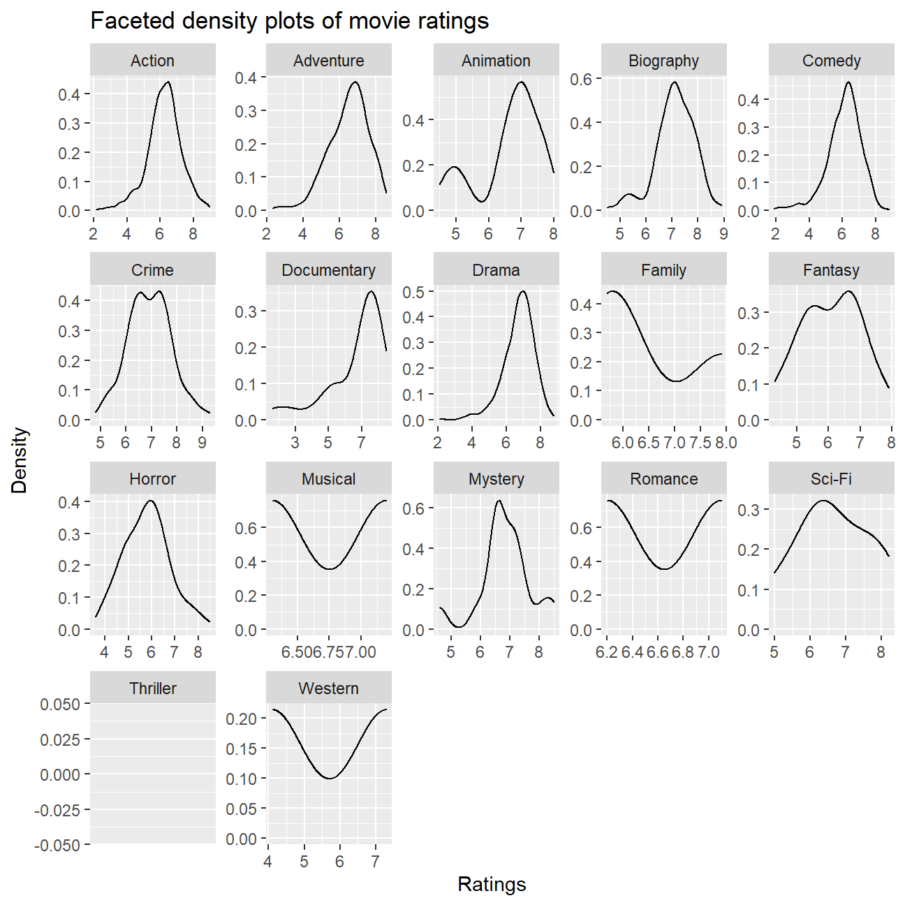
# Faceted density plots are not as effective or accurate because we earlier saw that there a select number of the genres (namely Sci-Fi, Family, Musical, Romance Western, Thriller) with especially few observations in them. The density function for those genres will thus not mean much.
# Notice also that the "Thriller" genre does not reflect any density plot because there was only one "Thriller" type movie within the entire dataset.

ggplot(cleaned_movies, aes(rating)) +
  geom_histogram() +
  facet_wrap(~ genre, scales = "free") +
  labs(title = "Faceted histogram plots of movie ratings", x = "Ratings", y = "Count")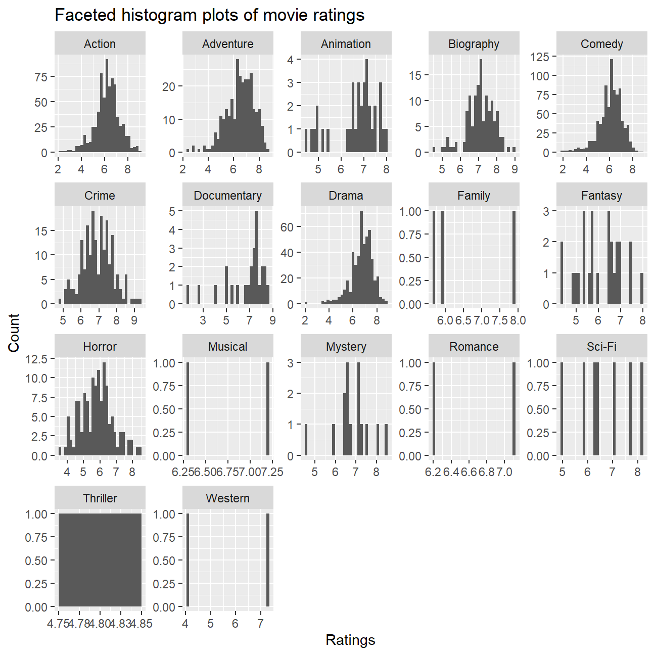
# The histogram plot is able to reflect much of the distribution.

ggplot(cleaned_movies, aes(rating)) +
    geom_histogram(aes(y=..density..),      # Histogram with density instead of count on y-axis
                   colour="black", fill="white") +
    geom_density(alpha=.2, fill="#FF6666") +  # Overlay with transparent density plot
    facet_wrap(~genre, scales = "free") +
    labs(title = "Faceted density plots overlaid on histograms of movie ratings", x = "Ratings", y = "Density")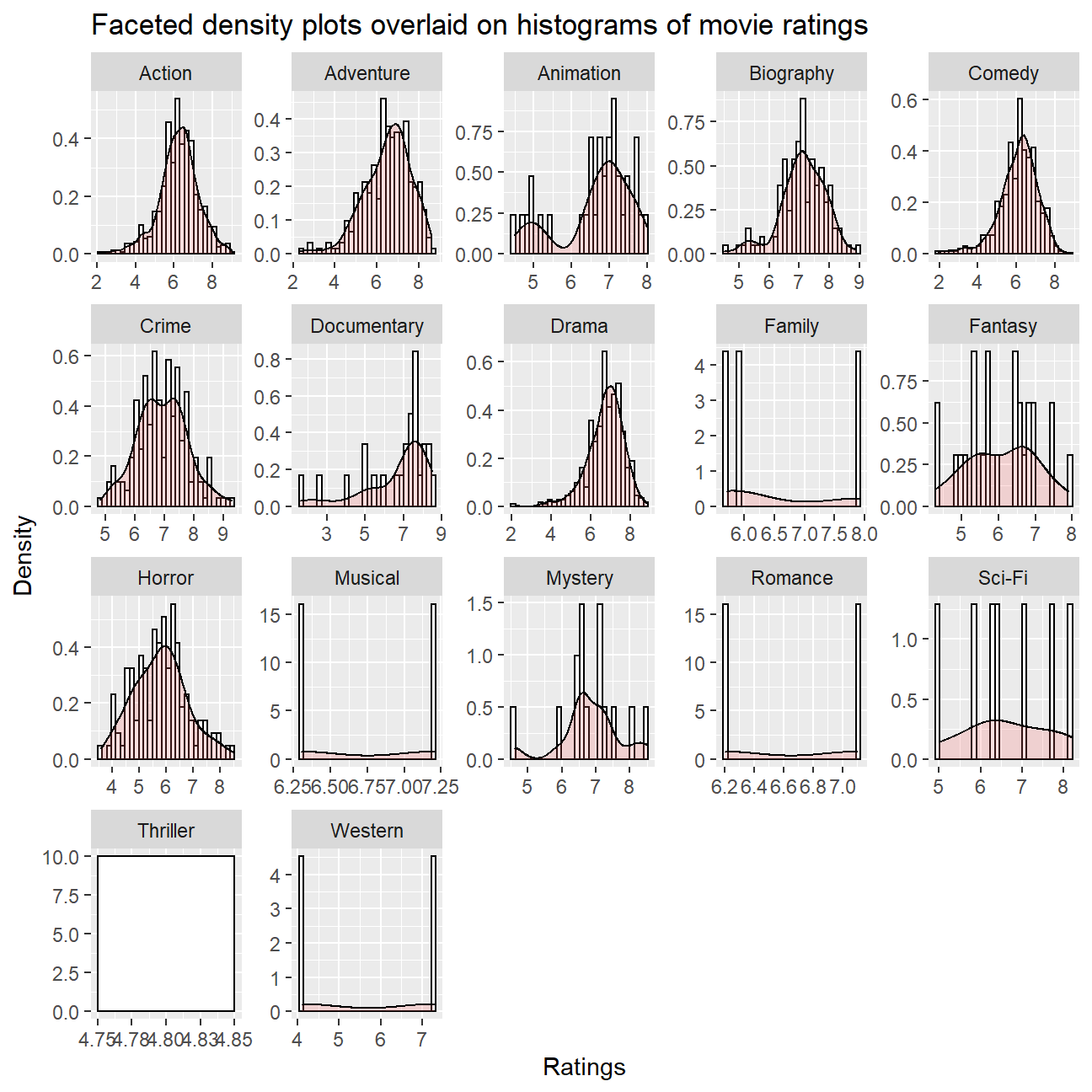
# To view an overlay of a density plot on histogram (done just out of interest)EDITOR’S NOTE:
The faceted density plots are not as effective or accurate because we earlier saw that there is a select number of the genres (namely Sci-Fi, Family, Musical, Romance Western, Thriller) with especially few observations in them. The density function for those genres will thus not mean much. Also, we noticed that the “Thriller” genre does not reflect any density plot because there was only one “Thriller” type movie within the entire dataset. The histogram plots, on the other hand, are able to showcase the distributions.
Use ggplot to answer the following
- Examine the relationship between
grossandcast_facebook_likes. Produce a scatterplot and write one sentence discussing whether the number of facebook likes that the cast has received is likely to be a good predictor of how much money a movie will make at the box office. What variable are you going to map to the Y- and X- axes?
# Plot total gross on number of facebook likes
ggplot(cleaned_movies, aes(cast_facebook_likes, gross, colour = genre)) +
  geom_point() +
  geom_smooth(se = FALSE)+
  xlim(0, 200000) + # Limit the x-scale to make the interpretation simpler
  scale_x_continuous(labels = ~ format(.x, scientific = FALSE)) +
  scale_y_continuous(labels = ~ format(.x, scientific = FALSE)) +
  labs(title = "Scatterplot of total gross amount on number of facebook likes", x = "Number of Facebook Likes", y = "Gross") +
  theme(legend.key.size = unit(0.5, 'cm'), #change legend key size
        legend.key.height = unit(0.5, 'cm'), #change legend key height
        legend.key.width = unit(0.5, 'cm'), #change legend key width
        legend.title = element_text(size=10), #change legend title font size
        legend.text = element_text(size=8))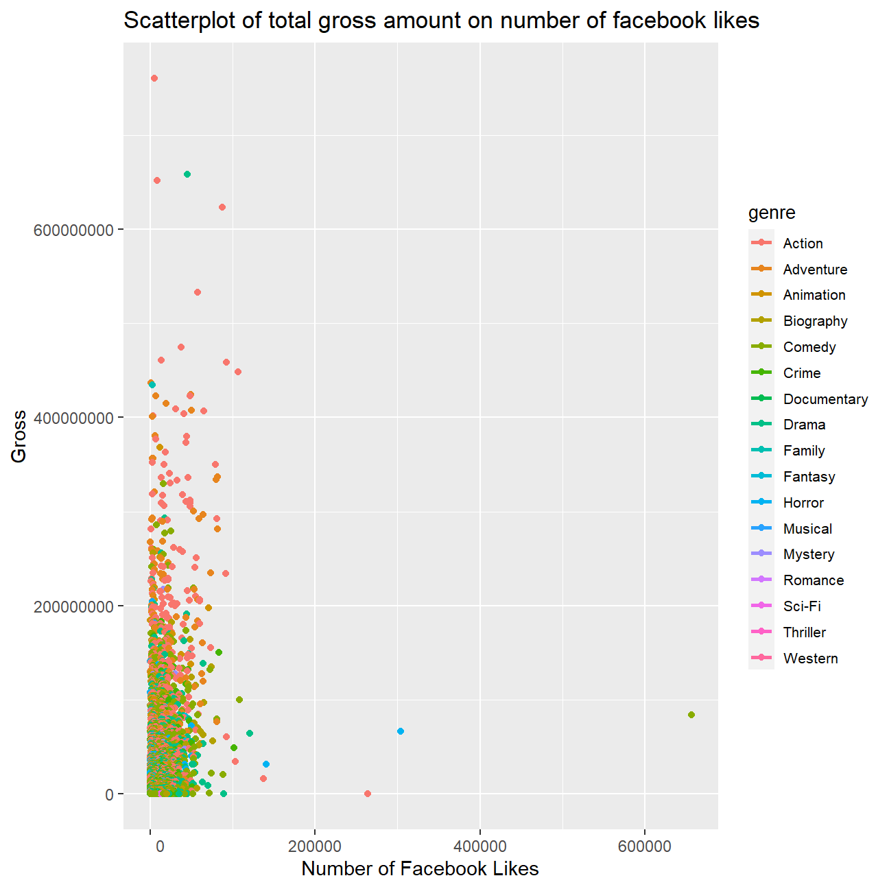
# As a sanity check, regress total gross on number of facebook likes
model <- lm(gross ~ cast_facebook_likes, data = cleaned_movies)
summary(model)
##
## Call:
## lm(formula = gross ~ cast_facebook_likes, data = cleaned_movies)
##
## Residuals:
## Min 1Q Median 3Q Max
## -4.45e+08 -4.33e+07 -2.22e+07 1.73e+07 7.08e+08
##
## Coefficients:
## Estimate Std. Error t value Pr(>|t|)
## (Intercept) 4.86e+07 1.53e+06 31.8 <2e-16 ***
## cast_facebook_likes 7.31e+02 6.39e+01 11.4 <2e-16 ***
## ---
## Signif. codes: 0 '***' 0.001 '**' 0.01 '*' 0.05 '.' 0.1 ' ' 1
##
## Residual standard error: 70700000 on 2905 degrees of freedom
## Multiple R-squared: 0.0432, Adjusted R-squared: 0.0428
## F-statistic: 131 on 1 and 2905 DF, p-value: <2e-16Although there is a positive correlation between the two variables, we believe that the facebook likes are not likely to be a good predictor of the money the movie will make at the box office based on the variability of outcomes as seen in the scatter plot. To confirm our intuition we did a basic regression of the likes on the gross revenues. We realize that there is a positive correlation and the predictor is significant, but based on the small r-squared value of around 0.05 we conclude that the predictive power of the facebook likes is not high.
- Examine the relationship between
grossandbudget. Produce a scatterplot and write one sentence discussing whether budget is likely to be a good predictor of how much money a movie will make at the box office.
# Plot scatterplot of total gross on budget
ggplot(cleaned_movies, aes(budget, gross, colour = genre)) +
  geom_point(aes(alpha = 0.1)) +
  geom_smooth(se = FALSE) +
  scale_x_continuous(labels = ~ format(.x, scientific = FALSE)) +
  labs(title = "Scatterplot of total gross amount on budget", x = "Budget", y = "Gross") +
  theme(legend.key.size = unit(0.5, 'cm'), #change legend key size
        legend.key.height = unit(0.5, 'cm'), #change legend key height
        legend.key.width = unit(0.5, 'cm'), #change legend key width
        legend.title = element_text(size=12), #change legend title font size
        legend.text = element_text(size=10))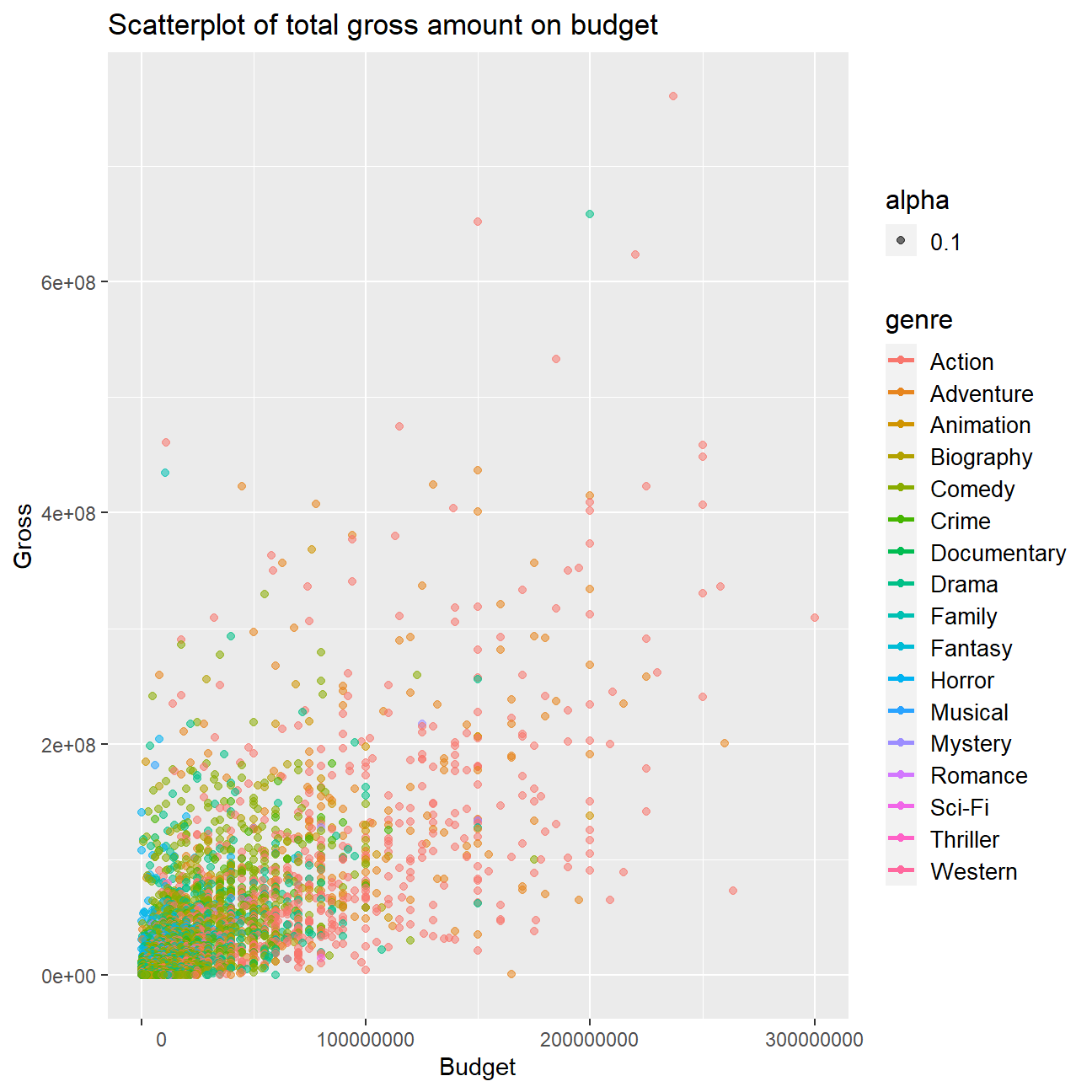
# As a sanity check, regress total gross on budget
model <- lm(gross ~ budget, data = movies)
summary(model)
##
## Call:
## lm(formula = gross ~ budget, data = movies)
##
## Residuals:
## Min 1Q Median 3Q Max
## -2.22e+08 -2.60e+07 -1.24e+07 1.31e+07 4.94e+08
##
## Coefficients:
## Estimate Std. Error t value Pr(>|t|)
## (Intercept) 1.49e+07 1.40e+06 10.7 <2e-16 ***
## budget 1.06e+00 2.34e-02 45.4 <2e-16 ***
## ---
## Signif. codes: 0 '***' 0.001 '**' 0.01 '*' 0.05 '.' 0.1 ' ' 1
##
## Residual standard error: 55600000 on 2959 degrees of freedom
## Multiple R-squared: 0.411, Adjusted R-squared: 0.41
## F-statistic: 2.06e+03 on 1 and 2959 DF, p-value: <2e-16The scatter plot displays a clear trend of higher budgets for movies being linked with higher gross revenues on box office. A simple linear regression confirms this positive relation with an r-squared value of 0.41 and a highly significant budget coefficient.
- Examine the relationship between
grossandrating. Produce a scatterplot, faceted bygenreand discuss whether IMDB ratings are likely to be a good predictor of how much money a movie will make at the box office. Is there anything strange in this dataset?
# Plot total gross on ratings
ggplot(cleaned_movies, aes(rating, gross, colour = factor(genre))) +
  geom_point(aes(alpha = 0.1)) +
  scale_x_continuous(labels = ~ format(.x, scientific = FALSE)) +
  ylim(0, 200000000) + # For clearer interpretation, we limit the y-scale
  facet_wrap(~ genre) +
  labs(title = "Scatterplot of total gross amount on rating", x = "Rating", y = "Gross") +
  theme(legend.key.size = unit(0.5, 'cm'), #change legend key size
        legend.key.height = unit(0.5, 'cm'), #change legend key height
        legend.key.width = unit(0.5, 'cm'), #change legend key width
        legend.title = element_text(size=12), #change legend title font size
        legend.text = element_text(size=10))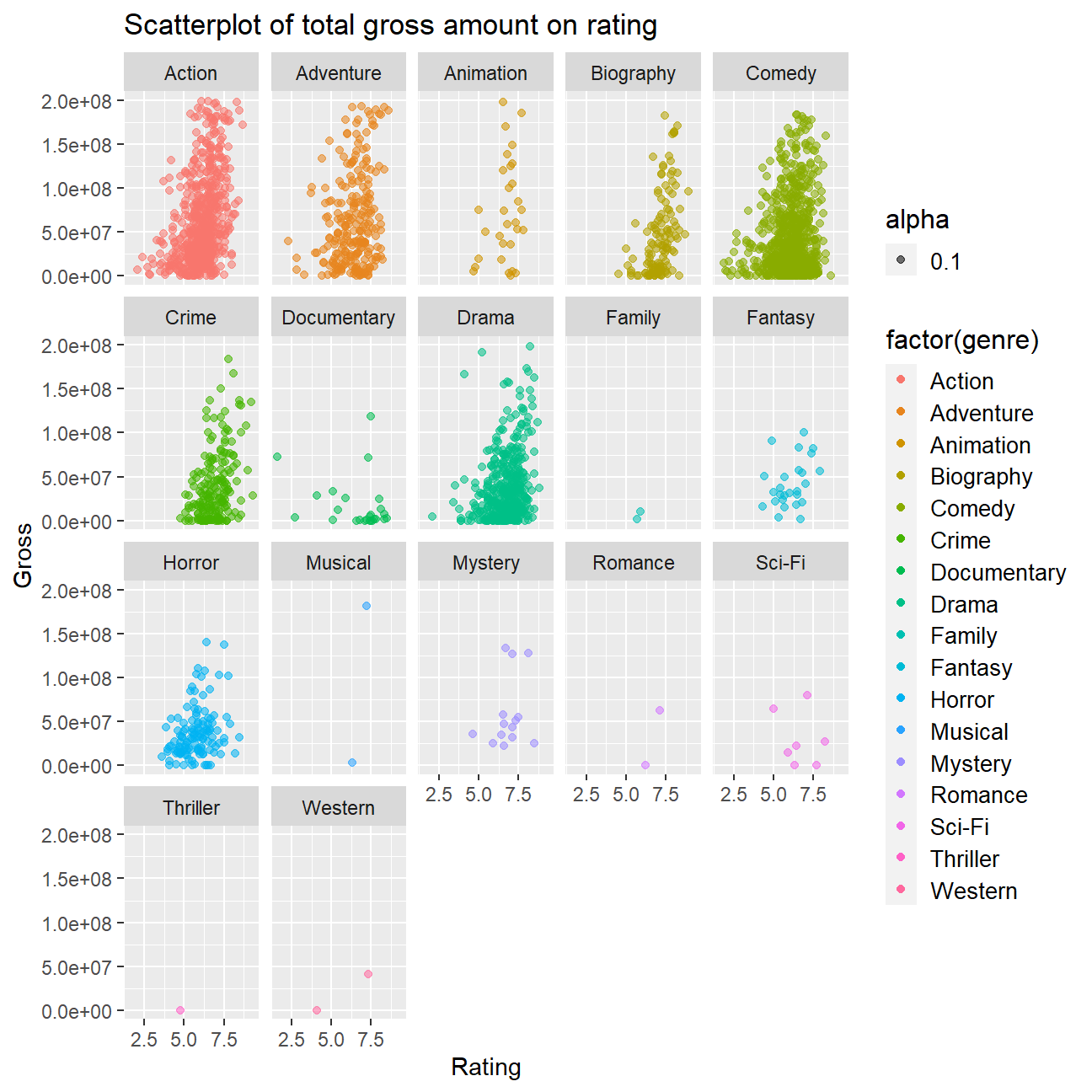
# As a sanity check, regress total gross on ratings
model <- lm(gross ~ rating, data = movies)
summary(model)
##
## Call:
## lm(formula = gross ~ rating, data = movies)
##
## Residuals:
## Min 1Q Median 3Q Max
## -98974277 -42915526 -17134877 19432831 674365127
##
## Coefficients:
## Estimate Std. Error t value Pr(>|t|)
## (Intercept) -60537478 7899673 -7.66 2.4e-14 ***
## rating 18566860 1219996 15.22 < 2e-16 ***
## ---
## Signif. codes: 0 '***' 0.001 '**' 0.01 '*' 0.05 '.' 0.1 ' ' 1
##
## Residual standard error: 69800000 on 2959 degrees of freedom
## Multiple R-squared: 0.0726, Adjusted R-squared: 0.0723
## F-statistic: 232 on 1 and 2959 DF, p-value: <2e-16When plotting the rating against the gross revenues for the movies, we can clearly identify a positive relation. However, there is a strong spread for given ratings. This is confirmed by our simple least squared regression, yielding an r-squared value 0.07. When braking it down by genre we noticed for genres such as action there a lot of movies and whilst better ratings seem to be reflected in higher gross revenues, there still remain big discrepancies for given ratings (e.g. for a similar rating, the revenue may differ 10-fold). For other genres, such as documentaries, there seems to be no positive correlation between ratings and gross revenues. Though, this might also be down to a small sample size.